")
In the last Blog, we explored the use of contour plots and other tools (such as a response optimizer) to help us quickly find solutions to our models. In this blog, we will look at the uncertainty in these predictions. We will also discuss model validation to ensure that technical assumptions that are inherent in the modeling process is satisfied.
We again start by revisiting the battery life DOE example that was discussed in the previous blog. Recall that previously we used the optimizer to find a solution for the wall thickness that would produce a target battery life of 45. As a reminder, we constrained the solution to use a Lithium battery since this made the response (battery life) insensitive to changes in ambient temperature. In the table below, we see that the wall thickness (uncoded) should be set at 1.44 (mm).
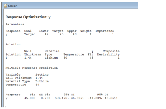
An important question with any model is how well does it predict? Suppose we actually produced a bunch of Lithium batteries with the wall thickness = 1.44. Would we always expect to get a battery life of exactly 45? The answer is NO!. Our model was not perfect (not all variation is explained) and even if it was, the model effects and parameters will based on average responses. The solution we found predicts that the average battery life will be 45.0 if we set wall thickness at 1.44.
At the bottom of the output above, we see both a 95% Confidence Interval (CI) and a 95% Prediction Interval (PI). The confidence interval tells us how much uncertainty exists in the average response. Thus, if we produce a lithium battery with a wall thickness of 1.44 mm, then we could expect that the range 43.475 to 46.525 has a 95% probability of containing the true average response. The prediction interval is always wider because it provided the range over which we may expect individual response values to fall. Thus, if we produce a lithium battery with a wall thickness of 1.44 mm, then we could expect that the range 41.339 to 48.661 has a 95% probability of containing the individual values. This is how much variation we could expect, given the uncertainty in our model. Note that the model uncertainty is both a function of the amount of data used to build the model as well as the experimental error observed in the study.
In the next blog, we will look a bit more at the uncertainty in these predictions. We will also, talk about model validation to ensure that technical assumptions that are inherent in this process are satisfied.
It is important to recognize the degree of uncertainty when using predictive models for making predictions, helping to set specifications, etc.
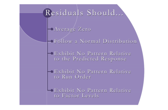
Next, let’s look at Model Validation. The basic reason for validating the model are summarized in the graphic below. To perform the validation, we calculate the residuals associated with each treatment.
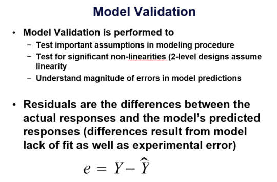
The residuals (errors) are calculated by any DOE software program, but they are not difficult to compute. We’ll look at a simple example.
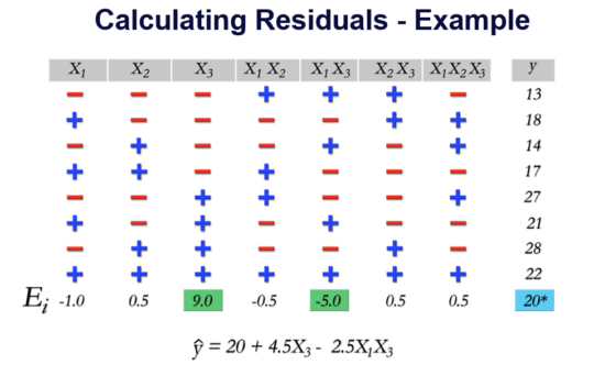
The experiment above is an experiment with 3 factors (2 levels). The right-most column contains the observed response and the model that was developed is shown at the bottom. (X3 and X1X3 were significant). For each row, we can plug in the actual coded values for X1 and X3 and compute the result, using the model. For the first row, both X1 and X3 are “low” (-1). So, we have:
y-hat = 20 + 4.5(-1) – 2.5(-1)(-1)
= 20 – 4.5 -2.5 = 13
Thus, the predicted value is 13 and the observed value is 13, so the residual is 13-13 = 0. The residuals for each row are calculated similarly.
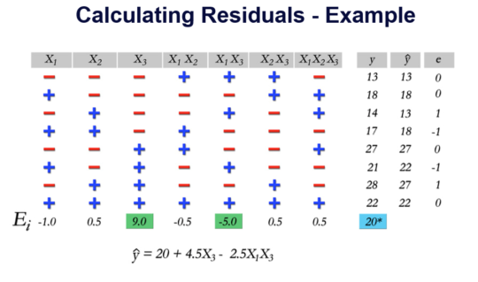
Once we compute all the residuals, we can determine how large they are and also graph them on various plots to determine if there are any significant violations of the model assumptions. The graphic below summarizes how residuals should behave if our modeling assumptions are satisfied.
Let’s consider some examples of residual plots.
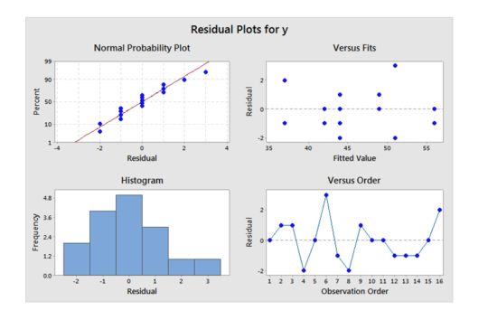
The upper left plot shows a normal probability plot which is used to check if residuals are reasonably described by a normal distribution. Since the points are close to linear on this plot, the normality assumption is satisfied. The upper right shows residuals vs. the model predicted values (fitted value). We are just looking for random values around zero and this one looks fine.
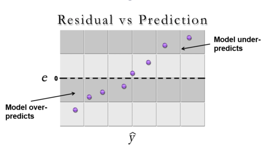
Let’s look at a few examples of model violations. In the plot below (residuals vs. predicted values) the module tends to over-predicts for smaller predicted values and under-predicts for larger predicted values. A valid model should not exhibit this pattern as it should predict similarly across the range of predicted values.
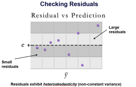
In the same kind of plot below, we see that the variability in residuals is not constant across the range of predicted values. This condition is called heterskedasticity, and means that the size of the model errors changes significantly across the range of predicted values. Constant variance of residuals is a requirement of the modeling method.
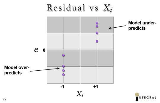
Below is a plot of residuals vs. the factor levels for a given factor. Just like across response levels, we shouldn’t see a pattern across factor levels.
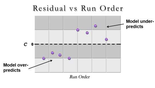
Finally, we should look at the residuals vs. the run order of the experiment. Non-random patterns may be indicative of a change occurring during the conduct of the experiment (assuming that the experiment was randomized). For example, in the plot below the first half of the runs look very different than the second half with regard to the predictive ability.
Violations of these rules may indicate non-linear responses, missing important factors, or other issues. Non-constant variances across the range or lack of normality can often be corrected by transforming the response values before developing the predictive model.
In the next blog, we will look at using Monte Carlo simulation with our predictive model to do some further optimization of target responses while considering variation in the factor levels.