An earlier article focused on the conceptual application of appropriate sample sizes for X-bar charts. As we discussed, the purpose of control charts is to detect significant process changes when they occur. When the proper sample size is selected, X-bar charts will detect process shifts (that have practical significance) in a timely manner.
In this article, we describe the sample size formula and its application in detail. The required sample size is a function of several variables that must either be estimated from the process or determined by the chart designer.
The formula for computing a sample size for an X-Bar chart is:
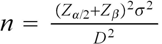
where:
n = sample size required
Za/2 = the number of standard deviations above zero on the standard normal distribution such that the area in the tail of the distribution is a/2 (a is the type I error probability and is typically 0.0027 for control chart applications. In this case, Z0.00135 = 3).
Zb = the number of standard deviations above zero on the standard normal distribution such that the area in the tail of the distribution is b (b is the type II error probability).
s = the standard deviation of the characteristic being charted.
D = the difference we are trying to detect.
The following factors influence the sample size:
- Type I error probability (a) – A Type I error occurs when we conclude that a control chart is giving us an out-of-control signal but the process is actually stable. This may be considered as a “false alarm.” In control chart applications, it is customary to set a = 0.0027. This is done so that the control limits trap 99.73% of the statistic that is being plotted on the control chart (note that 99.73% is trapped by placing control limits at ±3 standard deviations from the process average for normally distributed statistics such as sample averages). Because a is typically 0.0027, the formula term involving a is typically Z0.0027/2 = Z0.00135 = 3.
- Type II error probability (b) – A Type II error occurs when we fail to detect an out-of-control condition when the process is actually not stable. This is a serious error, as the whole purpose of the control chart is to detect a change quickly after the change occurs! As the Type II error is decreased, the required sample size to detect a process change increases (provided all other factors are unchanged). Once b is specified by the chart designer (a function of risk tolerance), Zb can be found from a standard normal table, which is available in any statistics textbook. The Microsoft EXCEL function:
=NORMSINV(1-b)
may also be utilized. Some common “Z values” are shown below:
Z0.00135 = 3
Z0.01 = 2.33
Z0.025 = 1.96
Z0.05 = 1.64
Z0.10 = 1.28
Z0.20 = 0.84
- The process standard deviation (s) – As the process standard deviation is decreased, the sample size required to detect a process change decreases (provided all other factors are unchanged). As the standard deviation increases, we need a large sample size to overcome the variation. s may be estimated from the process data. (See the earlier article on computing the standard deviation).
- The desired chart sensitivity (D) – D is the difference between the current process average and a new average, which represents a change that has practical significance. In other words, D represents the change in the process average that we are seeking to detect with the control chart. As the change we are trying to detect is decreased, the sample size required to detect a process change increases (provided all other factors are unchanged).
Selecting a sample size involves a trade-off between the above factors. Because for x-bar charts, the control limits are traditionally placed at ±3 standard deviations from the process average, the Type I error (a) is typically fixed at 0.0027. Furthermore, the process standard deviation (s), is typically estimated from the production process (rather than specified). This leaves us to trade off the chart sensitivity (D), the Type II error (b), and the required sample size (n). Increasing the sensitivity of the control chart (reducing D) or decreasing the probability of a Type II error both result in a larger required sample size.
Example:
Suppose that a beer bottler is filling containers labeled as 12 oz. The process standard deviation is estimated to be 0.12 ounces. The bottle weights follow a Normal distribution, so the bottler decides to center the process at 12.36 ounces to protect themselves against potential “underfills.” In addition the company is worried about overfilling, so the risk of a process shift is on both ends.
What sample size is required to detect a shift of 0.18 oz with 80% probability? (20% probability that the chart does not detect the shift).
We have:
Za/2 = Z0.00135 = 3
Zb = Z0.20 = 0.84
s = 0.12
D = 0.18 oz
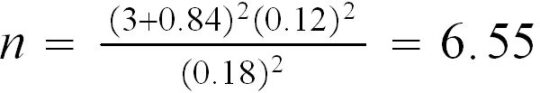
Thus, the required sample size is 7.
How does the required sample size change if we are only willing to tolerate a 10% chance that the chart fails to detect the shift? (Answer n = 8.14, so a sample size of 9 is required).